Danh sách package R phân tích dữ liệu

Biên soạn

Duc Nguyen | Founder of tuhocr.com

Cập nhật

2026 September 06

1 Mở đầu

R là ngôn ngữ lập trình để xử lý dữ liệu hàng đầu hiện nay, được thiết kế chuyên để xử lý thống kê và vẽ đồ thị. Đặc điểm của R là các câu lệnh được tối ưu để tính toán theo kiểu vector, ta có thể sử dụng các function từ gói package R Base mặc định cũng như từ các package chuyên môn (bản chất là các câu lệnh R được đóng gói thành function) để tính toán nhanh gọn một tác vụ xử lý dữ liệu cụ thể.

Bạn có thể tham khảo danh sách tổng hợp các package chuyên môn theo chủ đề được nhóm phát triển R Core Team tổng hợp ở đây CRAN Task Views.

Trong file HTML này mình tổng hợp các package và cụm lệnh thường sử dụng khi phân tích dữ liệu. Hy vọng sẽ hữu ích cho bạn để nhanh chóng áp dụng các package này vào công việc. Các bạn có thể đóng góp thêm cho danh sách được đầy đủ bằng cách chia sẻ trên Group Cộng Đồng Tự Học R nhé. Cảm ơn các bạn rất nhiều.

Để hiểu rõ hơn cách cài đặt package trong R, bạn xem video này nhé. Bài giảng.

Các câu lệnh nâng cao khi xử lý package trong R. Link.

2 R Base

Khi mở phiên làm việc (session) trong RStudio, bạn dùng câu lệnh sau sẽ liệt kê các package mặc định của R Base.

cat(search() , sep = "\n")

.GlobalEnv
package:dplyr
package:stats
package:graphics
package:grDevices
package:utils
package:datasets
package:methods
Autoloads
package:base

Các lệnh R cơ bản thường dùng được mình trình bày chi tiết trong khóa học R for Data Science. Link

Summary dữ liệu

aggregate(weight ~ group,
          x = PlantGrowth,
          FUN = mean)

  group weight
1  ctrl  5.032
2  trt1  4.661
3  trt2  5.526

3 Xử lý dữ liệu

3.1 Package `dplyr`

Đây là package được thiết kế theo phương thức lập trình dùng dấu %>% hay |> để đẩy kết quả phân tích từ bên trái qua tham số thứ nhất của function bên phải, thuận tiện tạo luồng code (chain), tái sử dụng đoạn code khi chỉ cần thay đổi dataset đầu vào.

Sắp xếp dữ liệu

library(dplyr)

# from small to big theo Girth
trees[1:6, ] |> dplyr:::arrange(Girth)

  Girth Height Volume
1   8.3     70   10.3
2   8.6     65   10.3
3   8.8     63   10.2
4  10.5     72   16.4
5  10.7     81   18.8
6  10.8     83   19.7

# from big to small theo Girth
trees[1:6, ] |> dplyr:::arrange(dplyr:::desc(Girth))

  Girth Height Volume
1  10.8     83   19.7
2  10.7     81   18.8
3  10.5     72   16.4
4   8.8     63   10.2
5   8.6     65   10.3
6   8.3     70   10.3

Summary dữ liệu

library(dplyr)

mtcars |> dplyr:::group_by(cyl) |> 
  dplyr:::summarise(mean_wt = mean(wt),
                    sd_wt = sd(wt),
                    count = dplyr:::n()) |> as.data.frame()

  cyl  mean_wt     sd_wt count
1   4 2.285727 0.5695637    11
2   6 3.117143 0.3563455     7
3   8 3.999214 0.7594047    14

4 Kỹ thuật lấy mẫu

4.1 Package `survey`

5 Phân tích thống kê

5.1 Package `car` và `effects`

Package này được viết bởi John Fox, sử dụng khi phân tích hồi quy. Chi tiết câu lệnh được hướng dẫn trong tài liệu An R Companion to Applied Regression. Link

Lệnh kiểm tra phân phối chuẩn bằng đồ thị QQ plot

par(pty = "s")
par(oma = c(0,0,0,0))
par(mar = c(2,4,0,2))

car:::qqPlot(mtcars$mpg)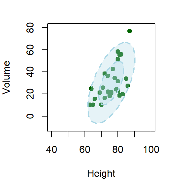

Vẽ đường mật độ xác suất ellipse

par(pty = "s")
par(oma = c(0,0,0,0))
par(mar = c(2,4,0,2))

plot(Volume ~ Height,
       data =  trees,
       col = "darkgreen",
       pch = 19,
      xlim = c(40,100),
       ylim = c(-10,80))

car:::dataEllipse.formula(Volume ~ Height,
                  data =  trees,
                 col = "lightblue",
                 pch = NA,
                 center.pch = FALSE,
                 fill = TRUE,
                 levels = c(0.5, 0.9),
                 fill.alpha = 0.3,
                 lty = 2,
                 add = T)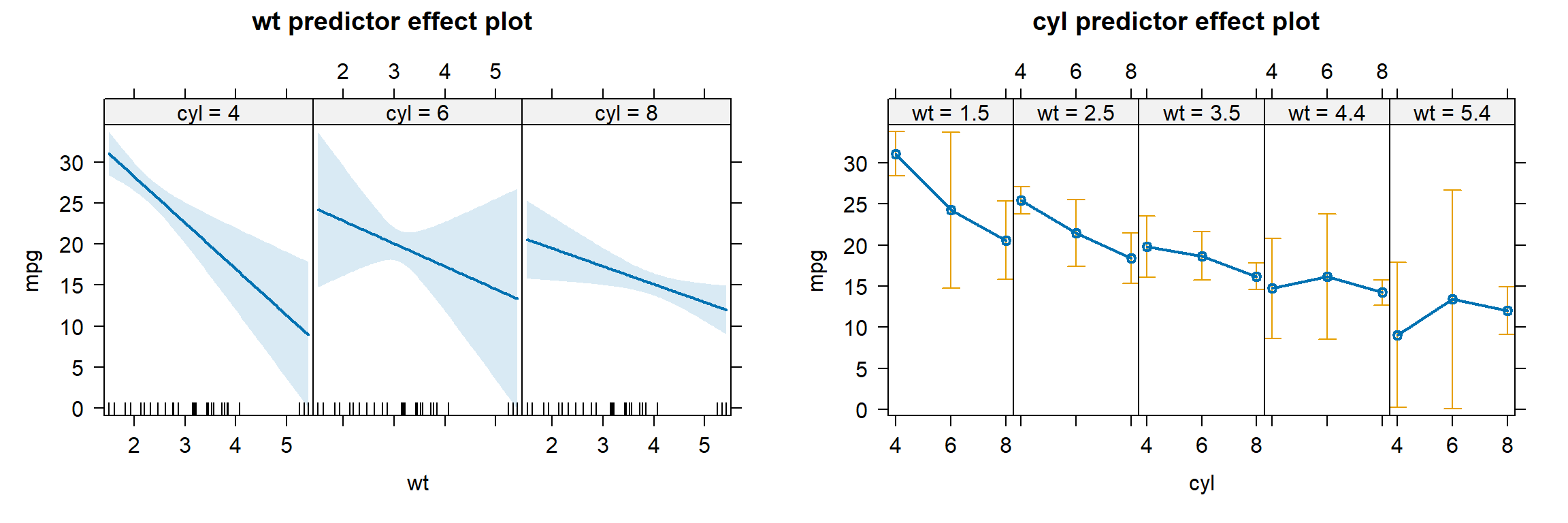

Vẽ đường effects plot | Vignettes

library(effects)

mtcars$cyl <- factor(mtcars$cyl)

fit <- lm(mpg ~ wt * cyl,
          data = mtcars)

effects:::plot.efflist(effects:::predictorEffects(fit),
                       lines = list(multiline = FALSE))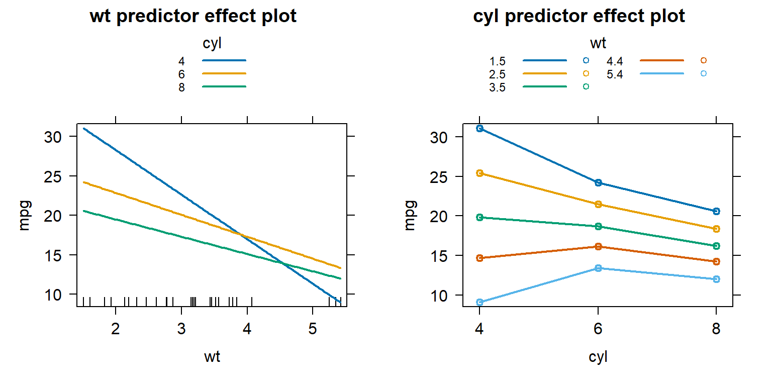

effects:::plot.efflist(effects:::predictorEffects(fit),
                       lines = list(multiline = TRUE))

6 Phân tích survival

6.1 Package `gtregression`

Ví dụ 1

Sử dụng bộ dữ liệu data_lungcancer trong package gtregression, ta có dataset sau. link

Hiển thị 10 dòng đầu tiên:

Code

library(gtregression)
library(dplyr)
library(gt)

data("data_lungcancer", package = "gtregression")

lung_data <- data_lungcancer |>
  mutate(
    treatment = factor(
      trt,
      levels = c(1, 2),
      labels = c("Standard", "Test")
    ),
    prior_therapy = factor(
      prior,
      levels = c(0, 10),
      labels = c("No", "Yes")
    )
  )

exposures <- c("treatment", "celltype", "karno", "age")

lung_data |>
  select(treatment, celltype, time, status, karno, age, prior_therapy) |>
  head(n=10)

   treatment celltype time status karno age prior_therapy
1   Standard squamous   72      1    60  69            No
2   Standard squamous  411      1    70  64           Yes
3   Standard squamous  228      1    60  38            No
4   Standard squamous  126      1    60  63           Yes
5   Standard squamous  118      1    70  65           Yes
6   Standard squamous   10      1    20  49            No
7   Standard squamous   82      1    40  69           Yes
8   Standard squamous  110      1    80  68            No
9   Standard squamous  314      1    50  43            No
10  Standard squamous  100      0    70  70            No

Tạo bảng survival

# hiển thị bảng HTML thì dùng results='asis' trong code chunk
km_summary <- gtregression:::survival_summary(
  data = lung_data,
  time = time,
  event = status,
  by = treatment,
  format = "gt"
)

km_summary

Group	N	Events	Censored	Median survival (95% CI)
Kaplan-Meier survival summary
Standard	69	64	5	103.0 (59.0-132.0)
Test	68	64	4	52.5 (44.0-95.0)
Median survival is estimated using Kaplan-Meier methods. Not reached means survival did not fall to 50% during observed follow-up.

Vẽ đường Kaplan–Meier

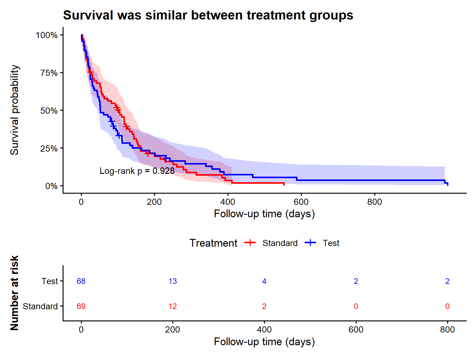
gtregression:::km_plot(
  data = lung_data,
  time = time,
  event = status,
  by = treatment,
  conf.int = T,
  risk_table = T,
  p_value = TRUE,
  break_time_by = 200,
  xlab = "Follow-up time (days)",
  title = "Survival was similar between treatment groups",
  legend_title = "Treatment",
  palette = c("red", "blue")
)

Cox model

Crude Cox model (model đơn biến)

cox_crude <- gtregression:::cox_reg(
  data = lung_data,
  time = time,
  event = status,
  exposures = c("treatment", "celltype", "karno", "age"),
  multivariable = F,
  format = "gt"
)

cox_crude

Characteristic	N	HR (95% CI)	p-value
treatment	137
Standard		Ref.
Test		1.02 (0.71–1.45)	0.922
celltype	137
squamous		Ref.
smallcell		2.72 (1.66–4.47)	<0.001
adeno		3.15 (1.77–5.59)	<0.001
large		1.26 (0.73–2.17)	0.407
karno	137	0.97 (0.96–0.98)	<0.001
age	137	1.01 (0.99–1.03)	0.433
Abbreviations: HR = Hazard Ratio; CI = Confidence Interval.
Ref. = reference category.

Multivariable Cox model (model đa biến)

cox_adjusted <- gtregression:::cox_reg(
  data = lung_data,
  time = time,
  event = status,
  exposures = c("treatment", "celltype", "karno", "age"),
  multivariable = TRUE,
  format = "gt"
)

cox_adjusted

Characteristic	Adjusted HR (95% CI)	p-value
treatment
Standard	Ref.
Test	1.35 (0.90–2.03)	0.141
celltype
squamous	Ref.
smallcell	2.35 (1.38–4.01)	0.002
adeno	3.25 (1.82–5.81)	<0.001
large	1.50 (0.86–2.60)	0.154
karno	0.97 (0.96–0.98)	<0.001
age	0.99 (0.97–1.01)	0.334
Abbreviations: HR = Hazard Ratio; CI = Confidence Interval.
Ref. = reference category.
Adjusted for the other variables in the model.

Check the proportional-hazards assumption

gtregression:::check_ph(cox_adjusted, format = "gt")

Model	Term	Test	Chi-square	df	p-value	Interpretation
Proportional hazards check
multivariable_model	treatment	Term	0.28	1	0.594	No evidence of PH violation
multivariable_model	celltype	Term	14.88	3	0.002	Possible PH violation
multivariable_model	karno	Term	12.98	1	<0.001	Possible PH violation
multivariable_model	age	Term	1.87	1	0.171	No evidence of PH violation
multivariable_model	GLOBAL	Global	29.18	6	<0.001	Possible PH violation
Screening aid only. Small p-values suggest possible non-proportional hazards; interpret with Schoenfeld residual plots, follow-up pattern, clinical context, and model purpose. alpha = 0.05; transform = km.

So sánh model

Dạng bảng

gtregression:::merge_tables(
  cox_crude,
  cox_adjusted,
  spanners = c("Crude", "Adjusted"),
  format = "gt"
)

Characteristic	Crude			Adjusted
Characteristic	N	HR (95% CI)	p-value	Adjusted HR (95% CI)	p-value
treatment	137
Standard		Ref.		Ref.
Test		1.02 (0.71–1.45)	0.922	1.35 (0.90–2.03)	0.141
celltype	137
squamous		Ref.		Ref.
smallcell		2.72 (1.66–4.47)	<0.001	2.35 (1.38–4.01)	0.002
adeno		3.15 (1.77–5.59)	<0.001	3.25 (1.82–5.81)	<0.001
large		1.26 (0.73–2.17)	0.407	1.50 (0.86–2.60)	0.154
karno	137	0.97 (0.96–0.98)	<0.001	0.97 (0.96–0.98)	<0.001
age	137	1.01 (0.99–1.03)	0.433	0.99 (0.97–1.01)	0.334
Abbreviations: HR = Hazard Ratio; CI = Confidence Interval.
Ref. = reference category.
Adjusted for the other variables in the model.

Dạng đồ thị

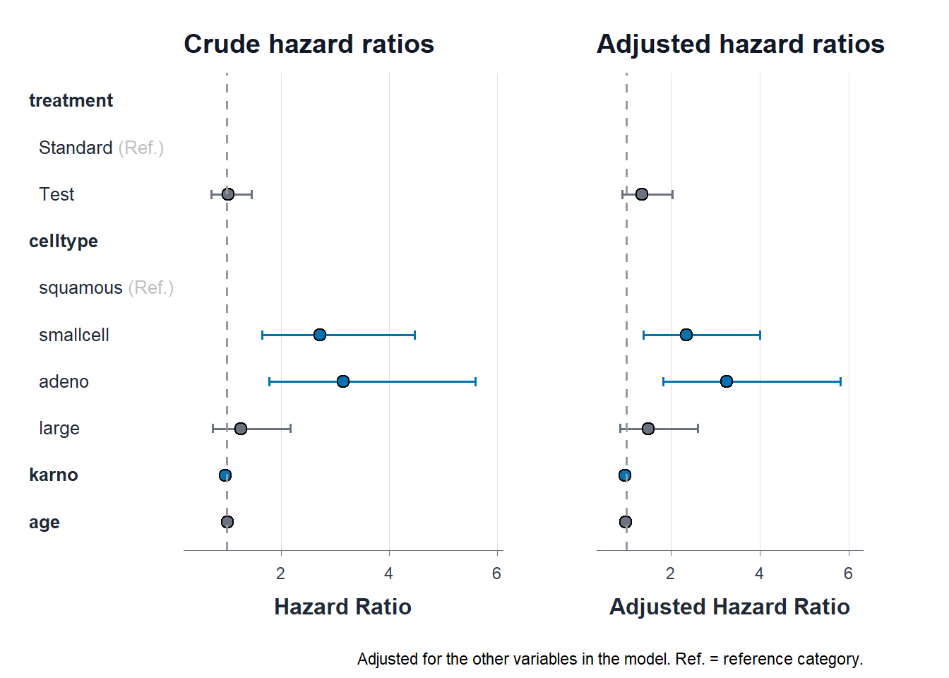
gtregression:::plot_reg_combine(
  cox_crude,
  cox_adjusted,
  title_uni = "Crude hazard ratios",
  title_multi = "Adjusted hazard ratios"
)

Forest plot

cox_forest_data <- gtregression:::forest_df(
  uni = cox_crude,
  multi = cox_adjusted
)

# cox_forest_data

cox_forest <- gtregression:::forest_reg(
  df = cox_forest_data,
  effects = c("Crude HR", "Adjusted HR"),
  ticks_at = c(0.5, 1, 2, 4)
)

gtregression:::save_forest(cox_forest,
                           "E:/GITHUB/thongkevavedothi/blog/package-r-data-science/cox_forest",
                           format = "png")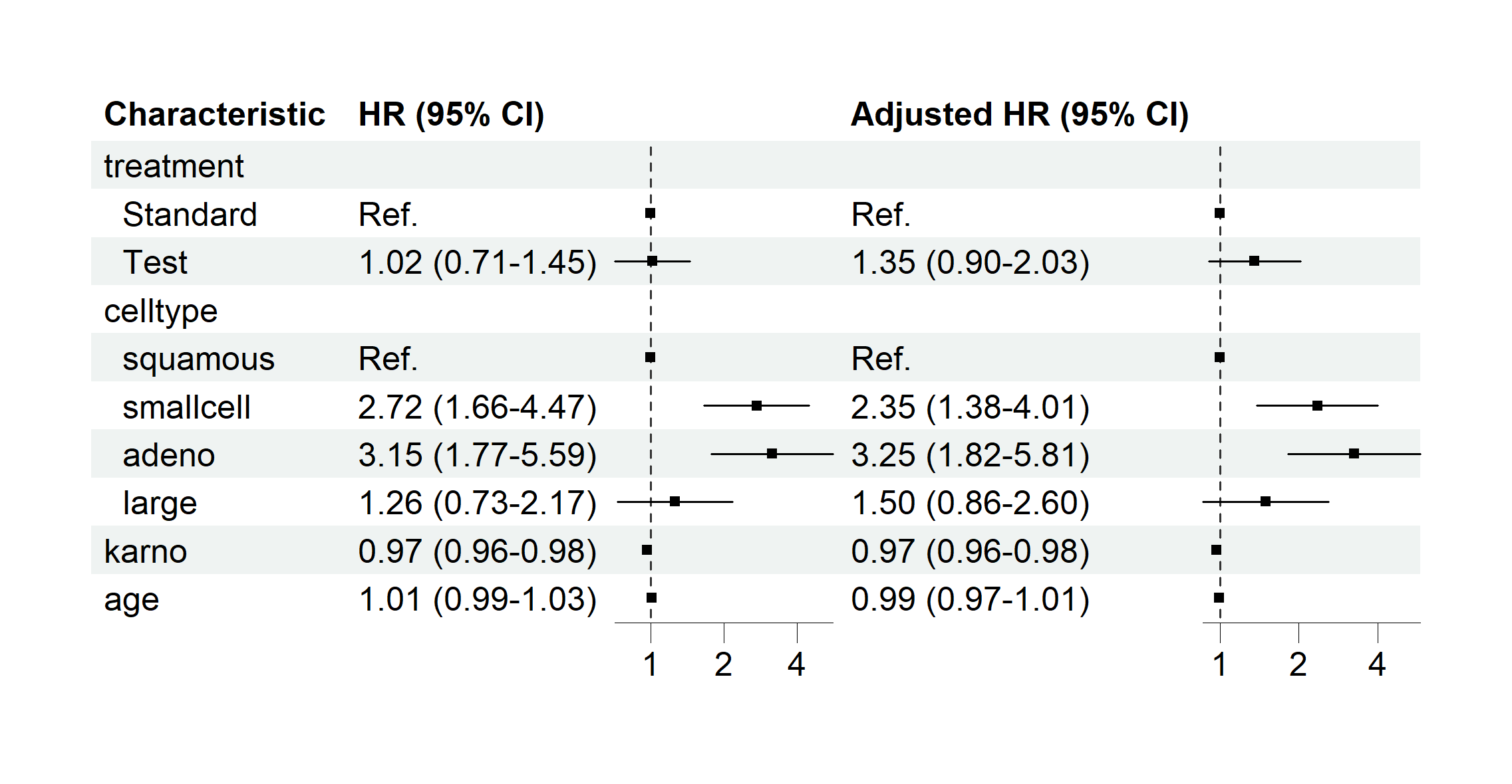

7 Machine learning

7.1 Package `caret`

8 Các lệnh làm việc với packge

Nhiều package có hiện tượng dùng trùng tên function, vì vậy ta nên khai báo triệt để đến namespace của function đó, bằng cách dùng dấu :::. Ví dụ muốn sử dụng function arrange() trong package dplyr, bạn nên dùng cú pháp sau dplyr:::arrange() để đảm bảo cho R dò tên function trong phạm vi package dplyr chứ không dùng nhầm qua package khác.

packageVersion("car")

install.packages("car")
remove.packages("car")

install.packages("https://cran.r-project.org/src/contrib/Archive/FAOSTAT/FAOSTAT_2.2.4.tar.gz",
                 repos = NULL,
                 type = "source")

library(devtools)
install_version("ggplot2", version = "0.9.1", repos = "http://cran.us.r-project.org")

# chỉ detach package và function thôi
unloadNamespace("plot.matrix")

detach("package:plot.matrix",
       unload = TRUE,
       force = TRUE)

### detach triệt để package và method đi kèm
pkgload:::unload("plot.matrix")
devtools::unload("plot.matrix")